Data processing with Pandas 2¶

Attention

Finnish university students are encouraged to use the CSC Notebooks platform.

Others can follow the lesson and fill in their student notebooks using Binder.

This week we will continue developing our skills using Pandas to process real data.

Motivation¶

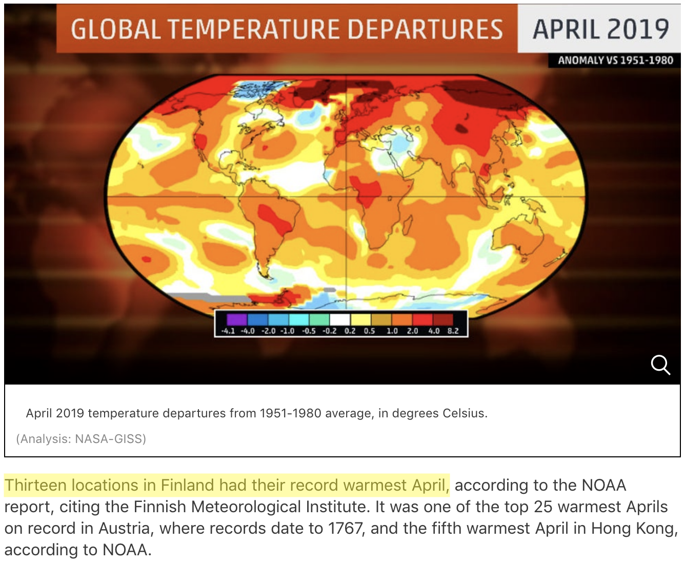Finland April 2019 Source: https://weather.com/news/climate/news/2019-05-20-april-2019-global-temperatures-nasa-noaa

April 2019 was the second warmest April on record globally, and the warmest on record at 13 weather stations in Finland. In this lesson, we will use our data manipulation and analysis skills to analyze weather data from Finland, and investigate the claim that April 2019 was the warmest on record across Finland.

Along the way we will cover a number of useful techniques in pandas including:

renaming columns
iterating data frame rows and applying functions
data aggregation
repeating the analysis task for several input files

Input data¶

In the lesson this week we are using weather observation data from Finland downloaded from NOAA. You will be working with data from either 15 or 4 different weather observation stations from Finland, depending on your environment.

Downloading the data¶

The first step for today’s lesson is to get the data. Which data files you download will depend on the platform you’re using for working through the lesson today. We recommend using the commandline tool wget for downloading the data. Wget is readily installed in the cloud computing environments.

CSC Notebooks users¶

Attention

It is recommended to use the Geo-Python Lite blueprint for this lesson if you would like to use data from all 15 weather observation stations.

First, you need to open a new terminal window in Jupyter Lab (from File -> New -> Terminal). Once the terminal window is open, you will need to navigate to the L6 directory:

cd notebooks/L6/

You can confirm that you are located in the correct directory by listing the contents of the current directory:

ls

You should see something like the following output:

advanced-data-processing-with-pandas.ipynb errors.ipynb                               img
debugging.ipynb                            gcp-5-assertions.ipynb

If so, you’re in the correct directory.

Downloading the data (Geo-Python Lite blueprint)¶

If you are using the Geo-Python Lite blueprint you can download the data using wget:

wget https://davewhipp.github.io/data/Finland-weather-data-full.tar.gz

After the download completes, you can extract the data files usign tar:

tar zxvf Finland-weather-data-full.tar.gz

At this stage you should have a new directory called data that contains the data for this week’s lesson. You can confirm this by listing the contents of the data-folder:

ls data

You should see something like the following:

028360.txt           029070.txt           029440.txt           029740.txt  6367598020644inv.txt
028690.txt           029110.txt           029500.txt           029810.txt  6367598020644stn.txt
028750.txt           029170.txt           029700.txt           029820.txt
028970.txt           029350.txt           029720.txt           3505doc.txt

Now you should be all set to proceed with the lesson!

Downloading the data (regular Geo-Python blueprint)¶

If you are using the regular Geo-Python blueprint you can download the data using wget:

wget https://davewhipp.github.io/data/Finland-weather-data-CSC.tar.gz

After the download completes, you can extract the data files using tar:

tar zxvf Finland-weather-data-CSC.tar.gz

At this stage you should have a new directory called data that contains the input data for this week’s lesson. You can confirm this by listing the contents of the data-folder:

ls data

You should see something like the following:

029440.txt           029720.txt           3505doc.txt          6367598020644stn.txt
029700.txt           029740.txt           6367598020644inv.txt

Now you should be all set to proceed with the lesson!

Students with Jupyter on their personal computers¶

If working on your own computer, you need to pay attention to the filepaths. First, you need to open a new terminal window in Jupyter Lab (from File -> New -> Terminal). Once the terminal window is open, you will need to navigate to the L6 directory:

cd path/to/L6/

where path/to/ should be replaced with the correct path for the Lesson 6 materials on your computer. Once in the correct directory, you can confirm this by typing:

ls

You should see something like the following output:

advanced-data-processing-with-pandas.ipynb errors.ipynb                               img
debugging.ipynb                            gcp-5-assertions.ipynb

Next, you can download the data files using wget:

wget https://davewhipp.github.io/data/Finland-weather-data-full.tar.gz

After the download completes, you can extract the data files usign tar:

tar zxvf Finland-weather-data-full.tar.gz

At this stage you should have a new directory called data that contains the data for this week’s lesson. You can confirm this by listing the contents of the data-folder:

ls data

You should see something like the following:

028360.txt           029070.txt           029440.txt           029740.txt  6367598020644inv.txt
028690.txt           029110.txt           029500.txt           029810.txt  6367598020644stn.txt
028750.txt           029170.txt           029700.txt           029820.txt
028970.txt           029350.txt           029720.txt           3505doc.txt

Now you should be all set to proceed with the lesson!

Binder users¶

It is not recommended to complete this lesson using Binder.

About the data¶

As part of the download there are a number of files that describe the weather data. These metadata files include:

A list of stations*: data/6367598020644stn.txt
Details about weather observations at each station: data/6367598020644inv.txt
A data description (i.e., column names): data/3505doc.txt

*Note that the list of stations is for all 15 stations, even if you’re working with only the 4 stations on the CSC Notebooks platform.

The input data for this week are separated with varying number of spaces (i.e., fixed width). The first lines and columns of the data look like following:

  USAF  WBAN YR--MODAHRMN DIR SPD GUS CLG SKC L M H  VSB MW MW MW MW AW AW AW AW W TEMP DEWP    SLP   ALT    STP MAX MIN PCP01 PCP06 PCP24 PCPXX SD
029440 99999 190601010600 090   7 *** *** OVC * * *  0.0 ** ** ** ** ** ** ** ** *   27 **** 1011.0 ***** ****** *** *** ***** ***** ***** ***** ** 
029440 99999 190601011300 ***   0 *** *** OVC * * *  0.0 ** ** ** ** ** ** ** ** *   27 **** 1015.5 ***** ****** *** *** ***** ***** ***** ***** ** 
029440 99999 190601012000 ***   0 *** *** OVC * * *  0.0 ** ** ** ** ** ** ** ** *   25 **** 1016.2 ***** ****** *** *** ***** ***** ***** ***** ** 
029440 99999 190601020600 ***   0 *** *** CLR * * *  0.0 ** ** ** ** ** ** ** ** *   26 **** 1016.2 ***** ****** *** *** ***** ***** ***** ***** **

We will develop our analysis workflow using data for a single station. Then, we will repeat the same process for all the stations.

Reading the data¶

In order to get started, let’s import pandas:

import pandas as pd

At this point, you can already have a quick look at the input file 029440.txt for Tampere Pirkkala and how it is structured. We can notice at least two things we need to consider when reading in the data:

Input data structure

Delimiter: The data are separated with a varying amount of spaces. If you check out the documentation for the read_csv() method, you can see that there are two different ways of doing this. We can use either sep='\s+' or delim_whitespace=True (but not both at the same time). In this case, we prefer to use delim_whitespace parameter.
No Data values: No data values in the NOAA data are coded with varying number of *. We can tell pandas to consider those characters as NaNs by specifying na_values=['*', '**', '***', '****', '*****', '******'].

# Define relative path to the file
fp = r'data/029440.txt'

# Read data using varying amount of spaces as separator and specifying * characters as NoData values
data = pd.read_csv(fp, delim_whitespace=True, na_values=['*', '**', '***', '****', '*****', '******'])

Let’s see how the data looks by printing the first five rows with the head() function:

data.head()

	USAF	WBAN	YR--MODAHRMN	DIR	SPD	GUS	CLG	SKC	L	M	...	SLP	ALT	STP	MAX	MIN	PCP01	PCP06	PCP24	PCPXX	SD
0	29440	99999	190601010600	90.0	7.0	NaN	NaN	OVC	NaN	NaN	...	1011.0	NaN	NaN	NaN	NaN	NaN	NaN	NaN	NaN	NaN
1	29440	99999	190601011300	NaN	0.0	NaN	NaN	OVC	NaN	NaN	...	1015.5	NaN	NaN	NaN	NaN	NaN	NaN	NaN	NaN	NaN
2	29440	99999	190601012000	NaN	0.0	NaN	NaN	OVC	NaN	NaN	...	1016.2	NaN	NaN	NaN	NaN	NaN	NaN	NaN	NaN	NaN
3	29440	99999	190601020600	NaN	0.0	NaN	NaN	CLR	NaN	NaN	...	1016.2	NaN	NaN	NaN	NaN	NaN	NaN	NaN	NaN	NaN
4	29440	99999	190601021300	270.0	7.0	NaN	NaN	OVC	NaN	NaN	...	1015.6	NaN	NaN	NaN	NaN	NaN	NaN	NaN	NaN	NaN

5 rows × 33 columns

All seems ok. However, we won’t be needing all of the 33 columns for detecting warm temperatures in April. We can check all column names by running data.columns:

data.columns

Index(['USAF', 'WBAN', 'YR--MODAHRMN', 'DIR', 'SPD', 'GUS', 'CLG', 'SKC', 'L',
       'M', 'H', 'VSB', 'MW', 'MW.1', 'MW.2', 'MW.3', 'AW', 'AW.1', 'AW.2',
       'AW.3', 'W', 'TEMP', 'DEWP', 'SLP', 'ALT', 'STP', 'MAX', 'MIN', 'PCP01',
       'PCP06', 'PCP24', 'PCPXX', 'SD'],
      dtype='object')

A description for all these columns is available in the metadata file data/3505doc.txt.

Let’s read in the data one more time. This time, we will read in only some of the columns using the usecols parameter. Let’s read in columns that might be somehow useful to our analysis, or at least that contain some values that are meaningful to us, including the station name, timestamp, and data about wind and temperature: 'USAF','YR--MODAHRMN', 'DIR', 'SPD', 'GUS','TEMP', 'MAX', 'MIN'

# Read in only selected columns
data = pd.read_csv(fp, delim_whitespace=True, 
                   usecols=['USAF','YR--MODAHRMN', 'DIR', 'SPD', 'GUS','TEMP', 'MAX', 'MIN'], 
                   na_values=['*', '**', '***', '****', '*****', '******'])

# Check the dataframe
data.head()

	USAF	YR--MODAHRMN	DIR	SPD	GUS	TEMP	MAX	MIN
0	29440	190601010600	90.0	7.0	NaN	27.0	NaN	NaN
1	29440	190601011300	NaN	0.0	NaN	27.0	NaN	NaN
2	29440	190601012000	NaN	0.0	NaN	25.0	NaN	NaN
3	29440	190601020600	NaN	0.0	NaN	26.0	NaN	NaN
4	29440	190601021300	270.0	7.0	NaN	27.0	NaN	NaN

Okay so we can see that the data was successfully read to the DataFrame and we also seemed to be able to convert the asterisk (*) characters into NaN values.

Renaming columns¶

As we saw above some of the column names are a bit awkward and difficult to interpret. Luckily, it is easy to alter labels in a pandas DataFrame using the rename-function. In order to change the column names, we need to tell pandas how we want to rename the columns using a dictionary that lists old and new column names

Let’s first check again the current column names in our DataFrame:

data.columns

Index(['USAF', 'YR--MODAHRMN', 'DIR', 'SPD', 'GUS', 'TEMP', 'MAX', 'MIN'], dtype='object')

Dictionaries

A dictionary is a specific data structure in Python for storing key-value pairs. During this course, we will use dictionaries mainly when renaming columns in a pandas series, but dictionaries are useful for many different purposes! For more information about Python dictionaries, check out this tutorial.

We can define the new column names using a dictionary where we list “key: value” pairs, in which the original column name (the one which will be replaced) is the key and the new column name is the value.

Let’s change the following:
- YR--MODAHRMN to TIME
- SPD to SPEED
- GUS to GUST

# Create the dictionary with old and new names
new_names = {'YR--MODAHRMN': 'TIME', 'SPD': 'SPEED', 'GUS': 'GUST'}

# Let's see what the variable new_names look like
new_names

{'YR--MODAHRMN': 'TIME', 'SPD': 'SPEED', 'GUS': 'GUST'}

# Check the data type of the new_names variable
type(new_names)

dict

From above we can see that we have successfully created a new dictionary.

Now we can change the column names by passing that dictionary using the parameter columns in the rename() function:

# Rename the columns
data = data.rename(columns=new_names)

# Print the new columns
print(data.columns)

Index(['USAF', 'TIME', 'DIR', 'SPEED', 'GUST', 'TEMP', 'MAX', 'MIN'], dtype='object')

Perfect, now our column names are easier to understand and use.

Check your understanding¶

The temperature values in our data files are again in Fahrenheit. As you might guess, we will soon convert these temperatures in to Celsius. In order to avoid confusion with the columns, let’s rename the column TEMP to TEMP_F. Let’s also rename USAF to STATION_NUMBER.

# Solution
# Create the dictionary with old and new names
new_names = {'USAF':'STATION_NUMBER', 'TEMP': 'TEMP_F'}

# Rename the columns
data = data.rename(columns=new_names)

# Check the output
data.head()

	STATION_NUMBER	TIME	DIR	SPEED	GUST	TEMP_F	MAX	MIN
0	29440	190601010600	90.0	7.0	NaN	27.0	NaN	NaN
1	29440	190601011300	NaN	0.0	NaN	27.0	NaN	NaN
2	29440	190601012000	NaN	0.0	NaN	25.0	NaN	NaN
3	29440	190601020600	NaN	0.0	NaN	26.0	NaN	NaN
4	29440	190601021300	270.0	7.0	NaN	27.0	NaN	NaN

Data properties¶

As we learned last week, it’s always a good idea to check basic properties of the input data before proceeding with data analysis. Let’s check the:

Number of rows and columns:

data.shape

(74940, 8)

Top and bottom rows:

data.head()

	STATION_NUMBER	TIME	DIR	SPEED	GUST	TEMP_F	MAX	MIN
0	29440	190601010600	90.0	7.0	NaN	27.0	NaN	NaN
1	29440	190601011300	NaN	0.0	NaN	27.0	NaN	NaN
2	29440	190601012000	NaN	0.0	NaN	25.0	NaN	NaN
3	29440	190601020600	NaN	0.0	NaN	26.0	NaN	NaN
4	29440	190601021300	270.0	7.0	NaN	27.0	NaN	NaN

data.tail()

	STATION_NUMBER	TIME	DIR	SPEED	GUST	TEMP_F	MAX	MIN
74935	29440	201910012220	130.0	3.0	NaN	39.0	NaN	NaN
74936	29440	201910012250	110.0	3.0	NaN	37.0	NaN	NaN
74937	29440	201910012300	100.0	2.0	NaN	38.0	NaN	NaN
74938	29440	201910012320	100.0	3.0	NaN	37.0	NaN	NaN
74939	29440	201910012350	110.0	3.0	NaN	37.0	NaN	NaN

Data types of the columns:

data.dtypes

STATION_NUMBER      int64
TIME                int64
DIR               float64
SPEED             float64
GUST              float64
TEMP_F            float64
MAX               float64
MIN               float64
dtype: object

Descriptive statistics:

data.describe()

	STATION_NUMBER	TIME	DIR	SPEED	GUST	TEMP_F	MAX	MIN
count	74940.0	7.494000e+04	71794.000000	74488.000000	10271.000000	74933.000000	1900.000000	1901.000000
mean	29440.0	2.011518e+11	306.184222	7.143755	16.706747	42.348018	46.622105	37.624934
std	0.0	2.590599e+09	294.547944	4.665385	5.186162	17.382721	17.735917	16.878257
min	29440.0	1.906010e+11	10.000000	0.000000	11.000000	-22.000000	-2.000000	-16.000000
25%	29440.0	2.017072e+11	140.000000	5.000000	13.000000	30.000000	33.000000	28.000000
50%	29440.0	2.018041e+11	210.000000	7.000000	15.000000	41.000000	46.000000	37.000000
75%	29440.0	2.019011e+11	320.000000	9.000000	19.000000	56.000000	61.000000	51.000000
max	29440.0	2.019100e+11	990.000000	59.000000	43.000000	88.000000	88.000000	80.000000

Here we can see that there are varying number of observations per column (see the count information), because some of the columns have missing values.

Using your own functions in Pandas¶

Now it’s again time to convert temperatures from Fahrenheit to Celsius! Yes, we have already done this many times before, but this time we will learn how to apply our own functions to data in a pandas DataFrame.

We will define a function for the temperature conversion, and apply this function for each Celsius value on each row of the DataFrame. Output celsius values should be stored in a new column called TEMP_C.

We will first see how we can apply the function row-by-row using a for loop and then we will learn how to apply the method to all rows more efficiently all at once.

Defining the function¶

For both of these approaches, we first need to define our temperature conversion function from Fahrenheit to Celsius:

def fahr_to_celsius(temp_fahrenheit):
    """Function to convert Fahrenheit temperature into Celsius.

    Parameters
    ----------

    temp_fahrenheit: int | float
        Input temperature in Fahrenheit (should be a number)
        
    Returns
    -------
    
    Temperature in Celsius (float)
    """

    # Convert the Fahrenheit into Celsius
    converted_temp = (temp_fahrenheit - 32) / 1.8
    
    return converted_temp

Let’s test the function with some known value:

fahr_to_celsius(32)

0.0

Let’s also print out the first rows of our data frame to see our input data before further processing:

data.head()

	STATION_NUMBER	TIME	DIR	SPEED	GUST	TEMP_F	MAX	MIN
0	29440	190601010600	90.0	7.0	NaN	27.0	NaN	NaN
1	29440	190601011300	NaN	0.0	NaN	27.0	NaN	NaN
2	29440	190601012000	NaN	0.0	NaN	25.0	NaN	NaN
3	29440	190601020600	NaN	0.0	NaN	26.0	NaN	NaN
4	29440	190601021300	270.0	7.0	NaN	27.0	NaN	NaN

Iterating over rows¶

We can apply the function one row at a time using a for loop and the iterrows() method. In other words, we can use the iterrows() method and a for loop to repeat a process for each row in a Pandas DataFrame . Please note that iterating over rows is a rather inefficient approach, but it is still useful to understand the logic behind the iteration.

When using the iterrows() method it is important to understand that iterrows() accesses not only the values of one row, but also the index of the row as well.

Let’s start with a simple for loop that goes through each row in our DataFrame:

# Iterate over the rows
for idx, row in data.iterrows():
    
    # Print the index value
    print('Index:', idx)
    
    # Print the row
    print('Temp F:', row['TEMP_F'], "\n")
    
    break

Index: 0
Temp F: 27.0 

Breaking a loop

When developing a for loop, you don’t always need to go through the entire loop if you just want to test things out. The break statement in Python terminates the current loop whereever it is placed and we used it here just to test check out the values on the first row. With a large data, you might not want to print out thousands of values to the screen!

We can see that the idx variable indeed contains the index value at position 0 (the first row) and the row variable contains all the data from that given row stored as a pandas Series.

Let’s now create an empty column TEMP_C for the Celsius temperatures and update the values in that column using the fahr_to_celsius function we defined earlier:

# Create an empty float column for the output values
data['TEMP_C'] = 0.0

# Iterate over the rows 
for idx, row in data.iterrows():
    
    # Convert the Fahrenheit to Celsius
    celsius = fahr_to_celsius(row['TEMP_F'])
    
    # Update the value of 'Celsius' column with the converted value
    data.at[idx, 'TEMP_C'] = celsius

Reminder: .at or .loc?

Here, you could also use data.loc[idx, new_column] = celsius to achieve the same result.

If you only need to access a single value in a DataFrame, DataFrame.at is faster compared to DataFrame.loc, which is designed for accessing groups of rows and columns.

Finally, let’s see how our dataframe looks like now:

data.head()

	STATION_NUMBER	TIME	DIR	SPEED	GUST	TEMP_F	MAX	MIN	TEMP_C
0	29440	190601010600	90.0	7.0	NaN	27.0	NaN	NaN	-2.777778
1	29440	190601011300	NaN	0.0	NaN	27.0	NaN	NaN	-2.777778
2	29440	190601012000	NaN	0.0	NaN	25.0	NaN	NaN	-3.888889
3	29440	190601020600	NaN	0.0	NaN	26.0	NaN	NaN	-3.333333
4	29440	190601021300	270.0	7.0	NaN	27.0	NaN	NaN	-2.777778

Applying the function¶

Pandas DataFrames and Series have a dedicated method .apply() for applying functions on columns (or rows!). When using .apply(), we pass the function name (without parenthesis!) as an argument to the apply() method. Let’s start by applying the function to the TEMP_F column that contains the temperature values in Fahrenheit:

data['TEMP_F'].apply(fahr_to_celsius)

     -2.777778
     -2.777778
     -3.888889
     -3.333333
     -2.777778
           ...   
  3.888889
  2.777778
  3.333333
  2.777778
  2.777778
Name: TEMP_F, Length: 74940, dtype: float64

The results look logical and we can store them permanently into a new column (overwriting the old values):

data['TEMP_C'] = data['TEMP_F'].apply(fahr_to_celsius)

We can also apply the function on several columns at once. We can re-order the dataframe at the same time in order to see something else than NaN from the MIN and MAX columns

data[['TEMP_F', 'MIN', 'MAX']].apply(fahr_to_celsius)

	TEMP_F	MIN	MAX
0	-2.777778	NaN	NaN
1	-2.777778	NaN	NaN
2	-3.888889	NaN	NaN
3	-3.333333	NaN	NaN
4	-2.777778	NaN	NaN
...	...	...	...
74935	3.888889	NaN	NaN
74936	2.777778	NaN	NaN
74937	3.333333	NaN	NaN
74938	2.777778	NaN	NaN
74939	2.777778	NaN	NaN

74940 rows × 3 columns

Check your understanding¶

Convert 'TEMP_F', 'MIN', 'MAX' to Celsius by applying the function like we did above and store the outputs to new columns 'TEMP_C', 'MIN_C', 'MAX_C'.

# Solution
data[['TEMP_C', 'MIN_C', 'MAX_C']]  = data[['TEMP_F', 'MIN', 'MAX']].apply(fahr_to_celsius)

Applying the function on all columns data.apply(fahr_to_celsius) would not give an error in our case, but the results also don’t make much sense for columns where input data was other than Fahrenheit temperatures.

You might also notice that our conversion function would also allow us to pass one column or the entire dataframe as a parameter. For example, like this: fahr_to_celsius(data["TEMP_F"]). However, the code is perhaps easier to follow when using the apply method.

Let’s check the output:

data.head(10)

	STATION_NUMBER	TIME	DIR	SPEED	GUST	TEMP_F	MAX	MIN	TEMP_C	MIN_C	MAX_C
0	29440	190601010600	90.0	7.0	NaN	27.0	NaN	NaN	-2.777778	NaN	NaN
1	29440	190601011300	NaN	0.0	NaN	27.0	NaN	NaN	-2.777778	NaN	NaN
2	29440	190601012000	NaN	0.0	NaN	25.0	NaN	NaN	-3.888889	NaN	NaN
3	29440	190601020600	NaN	0.0	NaN	26.0	NaN	NaN	-3.333333	NaN	NaN
4	29440	190601021300	270.0	7.0	NaN	27.0	NaN	NaN	-2.777778	NaN	NaN
5	29440	190601022000	NaN	0.0	NaN	27.0	NaN	NaN	-2.777778	NaN	NaN
6	29440	190601030600	270.0	7.0	NaN	26.0	NaN	NaN	-3.333333	NaN	NaN
7	29440	190601031300	270.0	7.0	NaN	25.0	NaN	NaN	-3.888889	NaN	NaN
8	29440	190601032000	270.0	7.0	NaN	24.0	NaN	NaN	-4.444444	NaN	NaN
9	29440	190601040600	NaN	0.0	NaN	18.0	NaN	NaN	-7.777778	NaN	NaN

Should I use .iterrows() or .apply()?

We are teaching the .iterrows() method because it helps to understand the structure of a DataFrame and the process of looping through DataFrame rows. However, using .apply() is often more efficient in terms of execution time.

At this point, the most important thing is that you understand what happens when you are modifying the values in a pandas DataFrame. When doing the course exercises, either of these approaches is ok!

Parsing dates¶

We will eventually want to group our data based on month in order to see if April temperatures in 2019 were higher than average. Currently, the date and time information is stored in the column TIME (which was originally titled YR--MODAHRMN:

YR--MODAHRMN = YEAR-MONTH-DAY-HOUR-MINUTE IN GREENWICH MEAN TIME (GMT)

Let’s have a closer look at the date and time information we have by checking the values in that column, and their data type:

data['TIME'].head(10)

  190601010600
  190601011300
  190601012000
  190601020600
  190601021300
  190601022000
  190601030600
  190601031300
  190601032000
  190601040600
Name: TIME, dtype: int64

data['TIME'].tail(10)

  201910012050
  201910012100
  201910012120
  201910012150
  201910012200
  201910012220
  201910012250
  201910012300
  201910012320
  201910012350
Name: TIME, dtype: int64

The TIME column contains several observations per day (and even several observations per hour). The timestamp for the first observation is 190601010600, i.e. from 1st of January 1906 (way back!), and the timestamp for the latest observation is 201910012350.

data['TIME'].dtypes

dtype('int64')

The information is stored as integer values.

We would want to aggregate the data on a monthly level, and in order to do so we need to “label” each row of data based on the month when the record was observed. In order to do this, we need to somehow separate information about the year and month for each row.

In practice, we can create a new column (or an index) containing information about the month (including the year, but excluding days, hours and minutes).

Before further processing, we want to convert the TIME column as character strings for convenience:

# Convert to string
data['TIME_STR'] = data['TIME'].astype(str)

String slicing¶

It is possible to convert the date and time information into character strings and “cut” the needed information from the string objects. If we look at the latest time stamp in the data (201910012350), you can see that there is a systematic pattern YEAR-MONTH-DAY-HOUR-MINUTE. Four first characters represent the year, and six first characters are year + month!

date = "201910012350"
date[0:6]

'201910'

Based on this information, we can slice the correct range of characters from the TIME_STR column using pandas.Series.str.slice()

# SLice the string
data['YEAR_MONTH'] = data['TIME_STR'].str.slice(start=0, stop=6)

# Let's see what we have
data.head()

	STATION_NUMBER	TIME	DIR	SPEED	GUST	TEMP_F	MAX	MIN	TEMP_C	MIN_C	MAX_C	TIME_STR	YEAR_MONTH
0	29440	190601010600	90.0	7.0	NaN	27.0	NaN	NaN	-2.777778	NaN	NaN	190601010600	190601
1	29440	190601011300	NaN	0.0	NaN	27.0	NaN	NaN	-2.777778	NaN	NaN	190601011300	190601
2	29440	190601012000	NaN	0.0	NaN	25.0	NaN	NaN	-3.888889	NaN	NaN	190601012000	190601
3	29440	190601020600	NaN	0.0	NaN	26.0	NaN	NaN	-3.333333	NaN	NaN	190601020600	190601
4	29440	190601021300	270.0	7.0	NaN	27.0	NaN	NaN	-2.777778	NaN	NaN	190601021300	190601

Nice! Now we have “labeled” the rows based on information about day of the year and hour of the day.

Check your understanding¶

Create a new column 'MONTH' with information about the month without the year.

# Solution
# Extract information about month from the TIME_STR column into a new column 'MONTH':
data['MONTH'] = data['TIME_STR'].str.slice(start=4, stop=6)

# Check the result
data[['YEAR_MONTH', 'MONTH']]

	YEAR_MONTH	MONTH
0	190601	01
1	190601	01
2	190601	01
3	190601	01
4	190601	01
...	...	...
74935	201910	10
74936	201910	10
74937	201910	10
74938	201910	10
74939	201910	10

74940 rows × 2 columns

Datetime (optional for Lesson 6)¶

In pandas, we can convert dates and times into a new data type datetime using pandas.to_datetime function.

# Convert character strings to datetime
data['DATE'] = pd.to_datetime(data['TIME_STR'])

# Check the output
data['DATE'].head()

 1906-01-01 06:00:00
 1906-01-01 13:00:00
 1906-01-01 20:00:00
 1906-01-02 06:00:00
 1906-01-02 13:00:00
Name: DATE, dtype: datetime64[ns]

Pandas Series datetime properties

There are several methods available for accessing information about the properties of datetime values. Read more from the pandas documentation about datetime properties.

Now, we can extract different time units based on the datetime-column using the pandas.Series.dt accessor:

data['DATE'].dt.year

      1906
      1906
      1906
      1906
      1906
         ... 
  2019
  2019
  2019
  2019
  2019
Name: DATE, Length: 74940, dtype: int64

data['DATE'].dt.month

       1
       1
       1
       1
       1
         ..
  10
  10
  10
  10
  10
Name: DATE, Length: 74940, dtype: int64

We can also combine the datetime functionalities with other methods from pandas. For example, we can check the number of unique years in our input data:

data['DATE'].dt.year.nunique()

For the final analysis, we need combined information of the year and month. One way to achieve this is to use the format parameter to define the output datetime format according to strftime(format) method:

# Convert to datetime and keep only year and month
data['YEAR_MONTH_DT'] = pd.to_datetime(data['TIME_STR'], format='%Y%m', exact=False)

exact=False finds the characters matching the specified format and drops out the rest (days, hours and minutes are excluded in the output).

data['YEAR_MONTH_DT']

     1906-01-01
     1906-01-01
     1906-01-01
     1906-01-01
     1906-01-01
           ...    
 2019-10-01
 2019-10-01
 2019-10-01
 2019-10-01
 2019-10-01
Name: YEAR_MONTH_DT, Length: 74940, dtype: datetime64[ns]

Now we have a unique label for each month as a datetime object.

Aggregating data in Pandas by grouping¶

Here, we will learn how to use pandas.DataFrame.groupby which is a handy method for compressing large amounts of data and computing statistics for subgroups.

We will use the groupby method to calculate the average temperatures for each month trough these main steps:

grouping the data based on year and month
Calculating the average for each month (each group)
Storing those values into a new DataFrame monthly_data

Before we start grouping the data, let’s once more check how our input data looks like:

print("number of rows:", len(data))

number of rows: 74940

data.head()

	STATION_NUMBER	TIME	DIR	SPEED	GUST	TEMP_F	MAX	MIN	TEMP_C	MIN_C	MAX_C	TIME_STR	YEAR_MONTH	MONTH	DATE	YEAR_MONTH_DT
0	29440	190601010600	90.0	7.0	NaN	27.0	NaN	NaN	-2.777778	NaN	NaN	190601010600	190601	01	1906-01-01 06:00:00	1906-01-01
1	29440	190601011300	NaN	0.0	NaN	27.0	NaN	NaN	-2.777778	NaN	NaN	190601011300	190601	01	1906-01-01 13:00:00	1906-01-01
2	29440	190601012000	NaN	0.0	NaN	25.0	NaN	NaN	-3.888889	NaN	NaN	190601012000	190601	01	1906-01-01 20:00:00	1906-01-01
3	29440	190601020600	NaN	0.0	NaN	26.0	NaN	NaN	-3.333333	NaN	NaN	190601020600	190601	01	1906-01-02 06:00:00	1906-01-01
4	29440	190601021300	270.0	7.0	NaN	27.0	NaN	NaN	-2.777778	NaN	NaN	190601021300	190601	01	1906-01-02 13:00:00	1906-01-01

We have quite a few rows of weather data, and several observations per day. Our goal is to create an aggreated data frame that would have only one row per month.

Let’s group our data based on unique year and month combinations

grouped = data.groupby('YEAR_MONTH')

Note

It would be also possible to create combinations of years and months on-the-fly when grouping the data:

# Group the data 
grouped = data.groupby(['YEAR', 'MONTH'])

Let’s explore the new variable grouped:

type(grouped)

pandas.core.groupby.generic.DataFrameGroupBy

len(grouped)

We have a new object with type DataFrameGroupBy with 82 groups. In order to understand what just happened, let’s also check the number of unique year and month combinations in our data:

data['YEAR_MONTH'].nunique()

Length of the grouped object should be the same as the number of unique values in the column we used for grouping. For each unique value, there is a group of data.

Let’s explore our grouped data further.

Check the “names” of each group

# Next line will print out all 82 group "keys"
#grouped.groups.keys()

Accessing data for one group:

Let’s check the contents for a group representing August 2019 (name of that group is (2019, 4) if you grouped the data based on datetime columns YEAR and MONTH). We can get the values of that hour from the grouped object using the get_group() method:

# Specify a month (as character string)
month = "190601"

# Select the group
group1 = grouped.get_group(month)

# Let's see what we have
group1

	STATION_NUMBER	TIME	DIR	SPEED	GUST	TEMP_F	MAX	MIN	TEMP_C	MIN_C	MAX_C	TIME_STR	YEAR_MONTH	MONTH	DATE	YEAR_MONTH_DT
0	29440	190601010600	90.0	7.0	NaN	27.0	NaN	NaN	-2.777778	NaN	NaN	190601010600	190601	01	1906-01-01 06:00:00	1906-01-01
1	29440	190601011300	NaN	0.0	NaN	27.0	NaN	NaN	-2.777778	NaN	NaN	190601011300	190601	01	1906-01-01 13:00:00	1906-01-01
2	29440	190601012000	NaN	0.0	NaN	25.0	NaN	NaN	-3.888889	NaN	NaN	190601012000	190601	01	1906-01-01 20:00:00	1906-01-01
3	29440	190601020600	NaN	0.0	NaN	26.0	NaN	NaN	-3.333333	NaN	NaN	190601020600	190601	01	1906-01-02 06:00:00	1906-01-01
4	29440	190601021300	270.0	7.0	NaN	27.0	NaN	NaN	-2.777778	NaN	NaN	190601021300	190601	01	1906-01-02 13:00:00	1906-01-01
...	...	...	...	...	...	...	...	...	...	...	...	...	...	...	...	...
88	29440	190601301300	320.0	9.0	NaN	12.0	NaN	NaN	-11.111111	NaN	NaN	190601301300	190601	01	1906-01-30 13:00:00	1906-01-01
89	29440	190601302000	320.0	9.0	NaN	19.0	NaN	NaN	-7.222222	NaN	NaN	190601302000	190601	01	1906-01-30 20:00:00	1906-01-01
90	29440	190601310600	320.0	11.0	NaN	14.0	NaN	NaN	-10.000000	NaN	NaN	190601310600	190601	01	1906-01-31 06:00:00	1906-01-01
91	29440	190601311300	320.0	14.0	NaN	20.0	NaN	NaN	-6.666667	NaN	NaN	190601311300	190601	01	1906-01-31 13:00:00	1906-01-01
92	29440	190601312000	360.0	5.0	NaN	21.0	NaN	NaN	-6.111111	NaN	NaN	190601312000	190601	01	1906-01-31 20:00:00	1906-01-01

93 rows × 16 columns

Ahaa! As we can see, a single group contains a DataFrame with values only for that specific month. Let’s check the DataType of this group:

type(group1)

pandas.core.frame.DataFrame

So, one group is a pandas DataFrame! This is really useful, because we can now use all the familiar DataFrame methods for calculating statistics etc for this specific group. We can, for example, calculate the average values for all variables using the statistical functions that we have seen already (e.g. mean, std, min, max, median, etc.).

We can do that by using the mean() function that we already used during Lesson 5.

Let’s calculate the mean for following attributes all at once:
- DIR,
- SPEED,
- GUST,
- TEMP,
- TEMP_C
- MONTH

# Specify the columns that will be part of the calculation
mean_cols = ['DIR', 'SPEED', 'GUST', 'TEMP_F', 'TEMP_C']

# Calculate the mean values all at one go
mean_values = group1[mean_cols].mean()

# Let's see what we have
print(mean_values)

DIR       218.181818
SPEED      13.204301
GUST             NaN
TEMP_F     25.526882
TEMP_C     -3.596177
dtype: float64

Here we saw how you can access data from a single group. For getting information about all groups (all months) we can use a for loop or methods available in the grouped object.

For loops and grouped objects:

When iterating over the groups in our DataFrameGroupBy object it is important to understand that a single group in our DataFrameGroupBy actually contains not only the actual values, but also information about the key that was used to do the grouping. Hence, when iterating over the data we need to assign the key and the values into separate variables.

Let’s see how we can iterate over the groups and print the key and the data from a single group (again using break to only see what is happening).

# Iterate over groups
for key, group in grouped:
    # Print key and group
    print("Key:\n", key)
    print("\nFirst rows of data in this group:\n", group.head())
    
    # Stop iteration with break command
    break

Key:
 190601

First rows of data in this group:
    STATION_NUMBER          TIME    DIR  SPEED  GUST  TEMP_F  MAX  MIN  \
         29440  190601010600   90.0    7.0   NaN    27.0  NaN  NaN   
         29440  190601011300    NaN    0.0   NaN    27.0  NaN  NaN   
         29440  190601012000    NaN    0.0   NaN    25.0  NaN  NaN   
         29440  190601020600    NaN    0.0   NaN    26.0  NaN  NaN   
         29440  190601021300  270.0    7.0   NaN    27.0  NaN  NaN   

     TEMP_C  MIN_C  MAX_C      TIME_STR YEAR_MONTH MONTH                DATE  \
-2.777778    NaN    NaN  190601010600     190601    01 1906-01-01 06:00:00   
-2.777778    NaN    NaN  190601011300     190601    01 1906-01-01 13:00:00   
-3.888889    NaN    NaN  190601012000     190601    01 1906-01-01 20:00:00   
-3.333333    NaN    NaN  190601020600     190601    01 1906-01-02 06:00:00   
-2.777778    NaN    NaN  190601021300     190601    01 1906-01-02 13:00:00   

  YEAR_MONTH_DT  
  1906-01-01  
  1906-01-01  
  1906-01-01  
  1906-01-01  
  1906-01-01  

Okey so from here we can see that the key contains the name of the group (year, month).

Let’s see how we can create a DataFrame where we calculate the mean values for all those weather attributes that we were interested in. I will repeat slightly the earlier steps so that you can see and better understand what is happening.

# Create an empty DataFrame for the aggregated values
monthly_data = pd.DataFrame()

# The columns that we want to aggregate
mean_cols = ['DIR', 'SPEED', 'GUST', 'TEMP_F', 'TEMP_C']

# Iterate over the groups
for key, group in grouped:
    
   # Calculate mean
   mean_values = group[mean_cols].mean()

   # Add the ´key´ (i.e. the date+time information) into the aggregated values
   mean_values['YEAR_MONTH'] = key

   # Append the aggregated values into the DataFrame
   monthly_data = monthly_data.append(mean_values, ignore_index=True)

Let’s see what we have now:

print(monthly_data)

           DIR      SPEED       GUST     TEMP_F     TEMP_C YEAR_MONTH
 218.181818  13.204301        NaN  25.526882  -3.596177     190601
 178.095238  13.142857        NaN  25.797619  -3.445767     190602
 232.043011  15.021505        NaN  22.806452  -5.107527     190603
 232.045455  13.811111        NaN  38.822222   3.790123     190604
 192.820513  10.333333        NaN  55.526882  13.070490     190605
..         ...        ...        ...        ...        ...        ...
370.992008   8.138490  17.251852  61.743400  16.524111     201906
294.433641   5.785714  15.034722  61.569955  16.427753     201907
320.335766   6.769447  15.751678  60.598649  15.888138     201908
306.491058   6.363594  15.173285  49.958137   9.976743     201909
239.577465  10.169014  17.470588  42.774648   5.985915     201910

[82 rows x 6 columns]

Awesome! Now we have aggregated our data and we have a new DataFrame called monthly_data where we have mean values for each month in the data set.

Mean for all groups at once

We can also achieve the same result by computing the mean of all columns for all groups in the grouped object:

grouped.mean()

	STATION_NUMBER	TIME	DIR	SPEED	GUST	TEMP_F	MAX	MIN	TEMP_C	MIN_C	MAX_C
YEAR_MONTH
190601	29440.0	1.906012e+11	218.181818	13.204301	NaN	25.526882	NaN	NaN	-3.596177	NaN	NaN
190602	29440.0	1.906021e+11	178.095238	13.142857	NaN	25.797619	NaN	NaN	-3.445767	NaN	NaN
190603	29440.0	1.906032e+11	232.043011	15.021505	NaN	22.806452	NaN	NaN	-5.107527	NaN	NaN
190604	29440.0	1.906042e+11	232.045455	13.811111	NaN	38.822222	NaN	NaN	3.790123	NaN	NaN
190605	29440.0	1.906052e+11	192.820513	10.333333	NaN	55.526882	NaN	NaN	13.070490	NaN	NaN
...	...	...	...	...	...	...	...	...	...	...	...
201906	29440.0	2.019062e+11	370.992008	8.138490	17.251852	61.743400	67.316667	55.600000	16.524111	13.111111	19.620370
201907	29440.0	2.019072e+11	294.433641	5.785714	15.034722	61.569955	67.774194	55.903226	16.427753	13.279570	19.874552
201908	29440.0	2.019082e+11	320.335766	6.769447	15.751678	60.598649	65.935484	55.016129	15.888138	12.786738	18.853047
201909	29440.0	2.019092e+11	306.491058	6.363594	15.173285	49.958137	53.766667	45.350000	9.976743	7.416667	12.092593
201910	29440.0	2.019100e+11	239.577465	10.169014	17.470588	42.774648	48.500000	41.000000	5.985915	5.000000	9.166667

82 rows × 11 columns

Detecting warm months¶

Now, we have aggregated our data on monthly level and all we need to do is to check which years had the warmest April temperatures. A simple approach is to select all Aprils from the data, group the data and check which group(s) have the highest mean value:

select all records that are from April (regardless of the year):

aprils = data[data['MONTH']=="04"]

take a subset of columns that might contain interesting information:

aprils = aprils[['STATION_NUMBER','TEMP_F', 'TEMP_C','YEAR_MONTH']]

group by year and month:

grouped = aprils.groupby(by='YEAR_MONTH')

calculate mean for each group:

monthly_mean = grouped.mean()

monthly_mean.head()

	STATION_NUMBER	TEMP_F	TEMP_C
YEAR_MONTH
190604	29440.0	38.822222	3.790123
190704	29440.0	36.111111	2.283951
190804	29440.0	36.811111	2.672840
190904	29440.0	31.977778	-0.012346
201704	29440.0	34.766620	1.537011

check the highest temperature values (sort the data frame in a descending order):

monthly_mean.sort_values(by='TEMP_C', ascending=False).head(10)

	STATION_NUMBER	TEMP_F	TEMP_C
YEAR_MONTH
201904	29440.0	42.472030	5.817794
201804	29440.0	38.951887	3.862159
190604	29440.0	38.822222	3.790123
190804	29440.0	36.811111	2.672840
190704	29440.0	36.111111	2.283951
201704	29440.0	34.766620	1.537011
190904	29440.0	31.977778	-0.012346

How did April 2019 rank at the Tampere Pirkkala observation station?

Repeating the data analysis with larger dataset¶

Finally, let’s repeat the data analysis steps above for all the available data we have (!!). First, confirm the path to the folder where all the input data are located. The idea is, that we will repeat the analysis process for each input file using a (rather long) for loop! Here we have all the main analysis steps with some additional output info - all in one long code cell:

# Read selected columns of  data using varying amount of spaces as separator and specifying * characters as NoData values
data = pd.read_csv(fp, delim_whitespace=True, 
                   usecols=['USAF','YR--MODAHRMN', 'DIR', 'SPD', 'GUS','TEMP', 'MAX', 'MIN'], 
                   na_values=['*', '**', '***', '****', '*****', '******'])

# Rename the columns
new_names = {'USAF':'STATION_NUMBER','YR--MODAHRMN': 'TIME', 'SPD': 'SPEED', 'GUS': 'GUST', 'TEMP':'TEMP_F'}
data = data.rename(columns=new_names)

#Print info about the current input file:
print("STATION NUMBER:", data.at[0,"STATION_NUMBER"])
print("NUMBER OF OBSERVATIONS:", len(data))

# Create column
col_name = 'TEMP_C'
data[col_name] = None

# Convert tempetarues from Fahrenheits to Celsius
data['TEMP_C'] = data['TEMP_F'].apply(fahr_to_celsius)

# Convert TIME to string 
data['TIME_STR'] = data['TIME'].astype(str)

# Parse year and month
data['MONTH'] = data['TIME_STR'].str.slice(start=5, stop=6).astype(int)
data['YEAR'] = data['TIME_STR'].str.slice(start=0, stop=4).astype(int)

# Extract observations for the months of April 
aprils = data[data['MONTH']==4]

# Take a subset of columns
aprils = aprils[['STATION_NUMBER','TEMP_F', 'TEMP_C', 'YEAR', 'MONTH']]

# Group by year and month
grouped = aprils.groupby(by=['YEAR', 'MONTH'])

# Get mean values for each group
monthly_mean = grouped.mean()

# Print info
print(monthly_mean.sort_values(by='TEMP_C', ascending=False).head(5))
print("\n")

STATION NUMBER: 29440
NUMBER OF OBSERVATIONS: 74940
            STATION_NUMBER     TEMP_F    TEMP_C
YEAR MONTH                                     
2019 4             29440.0  42.472030  5.817794
2018 4             29440.0  38.951887  3.862159
1906 4             29440.0  38.822222  3.790123
1908 4             29440.0  36.811111  2.672840
1907 4             29440.0  36.111111  2.283951

We will use the glob() function from the module glob to list our input files.

import glob

file_list = glob.glob(r'data/0*txt')

Note

Note that we’re using the * character as a wildcard, so any file that starts with data/0 and ends with txt will be added to the list of files we will iterate over. We specifically use data/0 as the starting part of the file names to avoid having our metadata files included in the list!

print("Number of files in the list", len(file_list))
print(file_list)

Number of files in the list 1
['data/029440.txt']

Now, you should have all the relevant file names in a list, and we can loop over the list using a for-loop:

for fp in file_list:
    print(fp)

data/029440.txt

# Repeat the analysis steps for each input file:
for fp in file_list:

    # Read selected columns of  data using varying amount of spaces as separator and specifying * characters as NoData values
    data = pd.read_csv(fp, delim_whitespace=True, usecols=['USAF','YR--MODAHRMN', 'DIR', 'SPD', 'GUS','TEMP', 'MAX', 'MIN'], na_values=['*', '**', '***', '****', '*****', '******'])

    # Rename the columns
    new_names = {'USAF':'STATION_NUMBER','YR--MODAHRMN': 'TIME', 'SPD': 'SPEED', 'GUS': 'GUST', 'TEMP':'TEMP_F'}
    data = data.rename(columns=new_names)

    #Print info about the current input file:
    print("STATION NUMBER:", data.at[0,"STATION_NUMBER"])
    print("NUMBER OF OBSERVATIONS:", len(data))

    # Create column
    col_name = 'TEMP_C'
    data[col_name] = None

    # Convert tempetarues from Fahrenheits to Celsius
    data['TEMP_C'] = data['TEMP_F'].apply(fahr_to_celsius)

    # Convert TIME to string 
    data['TIME_STR'] = data['TIME'].astype(str)

    # Parse year and month
    data['MONTH'] = data['TIME_STR'].str.slice(start=5, stop=6).astype(int)
    data['YEAR'] = data['TIME_STR'].str.slice(start=0, stop=4).astype(int)

    # Extract observations for the months of April 
    aprils = data[data['MONTH']==4]

    # Take a subset of columns
    aprils = aprils[['STATION_NUMBER','TEMP_F', 'TEMP_C', 'YEAR', 'MONTH']]

    # Group by year and month
    grouped = aprils.groupby(by=['YEAR', 'MONTH'])

    # Get mean values for each group
    monthly_mean = grouped.mean()

    # Print info
    print(monthly_mean.sort_values(by='TEMP_C', ascending=False).head(5))
    print("\n")

STATION NUMBER: 29440
NUMBER OF OBSERVATIONS: 74940

            STATION_NUMBER     TEMP_F    TEMP_C
YEAR MONTH                                     
4             29440.0  42.472030  5.817794
4             29440.0  38.951887  3.862159
4             29440.0  38.822222  3.790123
4             29440.0  36.811111  2.672840
4             29440.0  36.111111  2.283951

How about now, how did April 2019 rank across different stations?